Data generation
Overview
To examine variants associated with phenotypes backwards in time, we assembled a large ancient DNA dataset. Here we present new genomic data from 86 ancient individuals from Medieval and post-Medieval periods from Denmark (Extended Data Fig. 2, Supplementary Note 1 and Supplementary Table 1). The samples range in age from around the eleventh to the eighteenth century. We extracted ancient DNA from tooth cementum or petrous bone and shotgun sequenced the 86 genomes to a depth of genomic coverage ranging from 0.02× to 1.6× (mean of 0.39× and median of 0.27×). The genomes of the 86 new individuals were imputed using 1000 Genomes phased data as a reference panel by an imputation method designed for low-coverage genomes (GLIMPSE)51, and we also imputed 1,664 ancient genomes presented in the accompanying study2. Depending on the specific data quality requirements for the downstream analyses, we filtered out samples with poor coverage and variant sites with low minor allele frequency (MAF) and low imputation quality (average genotype probability of <0.98). Our dataset of ancient individuals spans approximately 15,000 years across Eurasia (Extended Data Fig. 2).
Authorizations for excavating the three sites, Kirkegård, Holbæk and Tjærby, were granted, respectively, to the Aalborg Historiske Museum, the Museum Vestsjælland (previously Museet for Holbæk og Omeg) and the Kulturhistorisk Museum Randers. The current study of samples from these three sites is covered by agreements given to GeoGenetics, Globe Institute, University of Copenhagen, by the Aalborg Historiske Museum, the Museum Vestsjælland and the Kulturhistorisk Museum Randers, respectively.
Ancient DNA extraction and library preparation
Laboratory work was conducted in the dedicated ancient DNA clean-room facilities at the Lundbeck Foundation GeoGenetics Centre (Globe Institute, University of Copenhagen). A total of 86 Medieval and post-Medieval human samples from Denmark (Supplementary Table 2) were processed using semi-automated procedures. Samples were processed in parallel. For each extract, non-USER-treated and USER-treated (NEB) libraries were built52. All libraries were sequenced on the NovaSeq 6000 instrument at the GeoGenetics Sequencing Core, Copenhagen, using S4 200-cycle kits v1.5. A more detailed description of DNA extraction and library preparation can be found in Supplementary Note 1.
Basic bioinformatics
The sequencing data were demultiplexed using the Illumina software BCL Convert (https://emea.support.illumina.com/sequencing/sequencing_software/bcl-convert.html). Adaptor sequences were trimmed and overlapping reads were collapsed using AdapterRemoval (v2.2.4)53. Single-end collapsed reads of at least 30 bp and paired-end reads were mapped to human reference genome build 37 using BWA (v0.7.17)54 with seeding disabled to allow for higher sensitivity. Paired- and single-end reads for each library and lane were merged, and duplicates were marked using Picard MarkDuplicates (v2.18.26; http://picard.sourceforge.net) with a pixel distance of 12,000. Read depth and coverage were determined using samtools (v1.10)55 with all sites used in the calculation (-a). Data were then merged to the sample level and duplicates were marked again.
DNA authentication
To determine the authenticity of the ancient reads, post-mortem DNA damage patterns were quantified using mapDamage2.0 (ref. 56). Next, two different methods were used to estimate the levels of contamination. First, we applied ContamMix to quantify the fraction of exogenous reads in the mitochondrial reads by comparing the mitochondrial DNA consensus genome to possible contaminant genomes57. The consensus was constructed using an in-house Perl script that used sites with at least 5× coverage, and bases were only called if observed in at least 70% of reads covering the site. Additionally, we applied ANGSD (v0.931)58 to estimate nuclear contamination by quantifying heterozygosity on the X chromosome in males. Both contamination estimates used only filtered reads with a base quality of ≥20 and mapping quality of ≥30.
Imputation
We combined the 86 newly sequenced Medieval and post-Medieval Danish individuals with 1,664 previously published ancient genomes2. We then excluded individuals showing contamination (more than 5%), low autosomal coverage (less than 0.1×) or low genome-wide average imputation genotype probability (less than 0.98), and we chose the higher-quality sample in a close relative pair (first- or second-degree relatives). A total of 1,557 individuals passed all filters and were used in downstream analyses. We restricted the analysis to SNPs with an imputation INFO score of ≥0.5 and MAF of ≥0.05.
Kinship analysis and uniparental haplogroup inference
READ59 was used to detect the degree of relatedness for pairs of individuals.
The mitochondrial DNA haplogroups of the Medieval and post-Medieval individuals were assigned using HaploGrep2 (ref. 60; Supplementary Fig. 3). Y-chromosome haplogroup assignment was inferred following an already published workflow61 (Supplementary Fig. 5). More details can be found in Supplementary Note 2.
Standard population genetics analyses
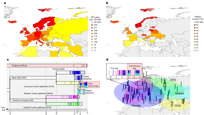
The main population genetics approach on which we based our inference was population-based painting (detailed below). However, to robustly understand population structure, we applied other standard techniques. First, we used principal-component analysis (PCA) (Extended Data Fig. 2) to investigate the overall population structure of the dataset. We used PLINK62, excluding SNPs with MAF < 0.05 in the imputed panel. On the basis of 1,210 ancient western Eurasian imputed genomes, the Medieval and post-Medieval samples clustered close to each other, displaying a relatively low genetic variability and situated within the genetic variability observed in the post-Bronze Age western Eurasian populations.
We then used two additional standard methods to estimate ancestry components in our ancient samples. First, we used model-based clustering (ADMIXTURE)63 (Supplementary Note 1 and Supplementary Fig. 1) on a subset of 826,248 SNPs. Second, we used qpAdm64 (Supplementary Note 1, Supplementary Fig. 2 and Supplementary Table 15) with a reference panel of three genetic ancestries (WHG, ANA and steppe) on the same 826,248 SNPs. We performed qpAdm applying the option ‘allsnps: YES’ and a set of seven outgroups was used as ‘right populations’: Siberia_UpperPaleolithic_UstIshim, Siberia_UpperPaleolithic_Yana, Russia_UpperPaleolithic_Sunghir, Switzerland_Mesolithic, Iran_Neolithic, Siberia_Neolithic and USA_Beringia. We set a minimum threshold of 100,000 SNPs, and only results with P < 0.05 were considered.
Population painting
Our main analysis used chromosome painting65 with a panel of six ancient ancestries. This allows fine-scale estimation of ancestry as a function of these populations. We ran chromosome painting on all ancient individuals not in the reference panel, using a reference panel of ancient donors grouped into populations to represent specific ancestries: WHG, EHG, CHG, farmer (ANA + Neolithic), steppe and African (method described in ref. 11). Painting followed the pipeline of ref. 66 based on GLOBETROTTER67, with admixture proportions estimated using NNLS. NNLS explains the genome-wide haplotype matches of an individual as a mixture of genome-wide haplotype matches of the reference populations. This set-up allows both the reference panel and any additional samples to be described using these six ancestries (Fig. 1).
We then painted individuals born in Denmark of a typical ancestry (typical on the basis of density-based clustering of the first 18 principal components11). The reference panel used for chromosome painting was designed to capture the various components of European ancestry only, and so we urge caution in interpreting these results for non-European samples.
This dataset provides the opportunity to study the population history of Denmark from the Mesolithic to the post-Medieval period, covering around 10,000 years, which can be considered a typical Northern European population. Our results clearly demonstrate the impact of previously described demographic events, including the influx of Neolithic farmer ancestry ~9,000 years ago and steppe ancestry ~5,000 years ago26,27. We highlight genetic continuity from the Bronze Age to the post-Medieval period (Supplementary Note 1 and Supplementary Fig. 1), although qpAdm detected a small increase in the farmer component during the Viking Age (Supplementary Note 1, Supplementary Fig. 2 and Supplementary Table 15), while the Medieval period marked a time of increased genetic diversity, probably reflecting increased mobility across Europe. This genetic continuity is further confirmed by the haplogroups identified in the uniparental genetic markers (Supplementary Note 2). Together, these results indicate that after the steppe migration in the Bronze Age there may have been no other major gene flow into Denmark from populations with significantly different Neolithic and Bronze Age ancestry compositions and therefore no changes in these ancestry components in the Danish population.
Local ancestry from population painting
Chromosome painting provides an estimate of the probability that an individual from each reference population is the closest match to the target individual at every position in the genome. This provided our first estimate of local ancestry from ref. 2: the population of the first reference individual to coalesce with the target individual, as estimated by Chromopainter65. This was estimated for all white British individuals in the UK Biobank, using the population painting reference panel described above. We refer to this as ‘local ancestry’, although we note that the closest relative in the sample may not represent ancestry in the conventional sense.
Pathway painting
An alternative approach is to identify to which of the four major ancestry pathways (ANA farmer, CHG, EHG and WHG) each position in the genome best matches. This has the advantage of not forcing haplotypes to choose between ‘steppe’ ancestry and its ancestors but the disadvantage of being more complex to interpret. To do this, we modelled ancestry path labels in the GBR, FIN and TSI 1000 Genomes populations68 and 1,015 ancient genomes generated using a neural network to assign ancestry paths on the basis of a sample’s nearest neighbours at the first five informative nodes of a marginal tree sequence, with an informative node defined as a node that had at least one leaf from the reference set of ancient samples described above (ref. 11; Supplementary Note 1c). We refer to these as ‘ancestry path labels’.
SNP associations
We aimed to generate SNP associations from previous studies for each phenotype in a consistent approach. To generate a list of SNPs associated with MS and RA, we used two approaches: in the first, we downloaded fine-mapped SNPs from previous association studies. For each fine-mapped SNP, if the SNP did not have an ancestry path label, we found the SNP with the highest LD that did, with a minimum threshold of r2 ≥ 0.7, in the GBR, FIN and TSI 1000 Genomes populations using LDLinkR69. The final SNPs used for each phenotype can be found in Supplementary Table 4 (MS) and Supplementary Table 5 (RA).
For MS, we used data from ref. 4. For non-MHC SNPs, we used the ‘discovery’ SNPs with P(joined) and OR(joined) generated in the replication phase. For MHC variants, we searched the literature for the reported HLA alleles and amino acid polymorphisms (Supplementary Table 3). In total, we generated 205 SNPs that were either fine-mapped or in high LD with a fine-mapped SNP (15 MHC, 190 non-MHC).
For RA, we downloaded 57 genome-wide-significant non-MHC SNPs for seropositive RA in Europeans70. We retrieved MHC associations separately (ref. 71; with associated ORs and P values from ref. 72). In total, we generated 51 SNPs that were either fine-mapped or in high LD with a fine-mapped SNP (3 MHC, 48 non-MHC).
Second, because we could not always find LD proxies for fine-mapped SNPs that were present in our ancestry path label dataset, we found that we were losing significant signal from the HLA region; therefore, we generated a second set of SNP associations. We downloaded full summary statistics for each disease (using ref. 4 for MS and ref. 73 for RA), restricted to sites present in the ancestry path label dataset, and ran PLINK’s (v1.90b4.4)74 clump method (parameters: –clump-p1 5e-8 –clump-r2 0.05 –clump-kb 250; as in ref. 75) using LD in the GBR, FIN and TSI 1000 Genomes populations68 to extract genome-wide-significant independent SNPs.
In the main text, we report results for the first set of SNPs (‘fine-mapped’) for analyses involving local ancestry in modern data and the second set of SNPs (‘pruned’) for analyses involving polygenic measures of selection (CLUES and PALM).
Anomaly score: regions of unusual ancestry
To assess which regions of ancestry were unusual, we converted the ancestry estimates to Z scores by standardizing to the genome-wide mean and standard deviation. Specifically, let A(i,j,k) denote the probability of the kth ancestry (k = 1, …, K) at the jth SNP (j = 1, …, J) of a chromosome for the ith individual (i = 1, …, N). We first computed the mean painting for each SNP, \(A\left(\right)=\frac{1}{N}{\sum }_{i=1}^{N}A\left(i,j,k\right)\). From this, we estimated a location parameter µk and a scale parameter σk using a block-median approach. Specifically, we partitioned the genome into 0.5-Mb regions and, within each, computed the mean and standard deviation of the ancestry. The parameter estimates were the median values over the whole genome. We then computed an anomaly score for each SNP for each ancestry Z(j,k) = (A(j,k) – µk)/σk. This is the normal-distribution approximation to the Poisson binomial score for excess ancestry, for which a detailed simulation study is presented in ref. 76.
To arrive at an anomaly score for each SNP aggregated over all ancestries, we also had to account for correlations in the ancestry paintings. Instead of scaling each ancestry deviation A*(j,k) = A(j,k) – µk by its standard deviation, we instead ‘whitened’ them, that is, rotated the data to have an independent signal. Let C = A*TA* be a K × K covariance matrix, and let C–1 = UDVT be a singular value decomposition. Then, \(W=U{D}^{\frac{1}{2}}\) is the whitening matrix from which Z = A*W is normally distributed with covariance matrix diag(1) under the null hypothesis that A* is normally distributed with mean 0 and unknown covariance Σ. The ancestry anomaly score test statistic for each SNP is \(t\left(\,j\right)={\sum }_{k=1}^{K}{Z\left(j,k\right)}^{2}\), which is chi-squared distributed with K degrees of freedom under the null, and we report P values from this.
To test for gene enrichment, we formed a list of all SNPs reaching genome-wide significance (P < 5 × 10⁻⁸) and, using the R package gprofiler2 (ref. 77), converted these to a list of unique genes. We then used gost to perform an enrichment test for each Gene Ontology (GO) term, for which we used default P-value correction via the g:Profiler SCS method. This is an empirical correction based on performing random lookups of the same number of genes under the null, to control the error rate and ensure that 95% of reported categories (at P = 0.05) are correct.
Allele frequency over time
To investigate how effect allele frequencies have changed over time, we extracted high-effect alleles for each phenotype from the ancient data. We excluded all non-Eurasian samples, grouped them by ‘groupLabel’, excluded any group with fewer than four samples and coloured points by ancestry proportion according to genome-wide NNLS based on chromosome painting (described above).
Weighted average prevalence
To understand whether risk-conferring haplotypes evolved in the steppe population or in a pre- or post-dating population, we developed a statistic that could account for the origin of risk to be identified with multiple ancestry groups, which do not have to be the same set for each SNP.
We first applied k-means clustering to the dosage of each ancestry for each associated SNP and investigated the dosage distribution of clusters with significantly higher MS prevalence. For the target SNPs, the elbow method78 suggested selecting around 5–7 clusters, and we chose 6 clusters. After performing the k-means cluster analysis, we calculated the average probability for each ancestry for case individuals. Furthermore, we calculated the prevalence of MS in each cluster and performed a one-sample t test to investigate whether it differed from the overall MS prevalence (0.487%). This tested whether any particular combinations of ancestry were associated with the phenotype at a SNP. Clusters with high MS risk ratios had a high proportion of steppe components (Supplementary Fig. 7), leading to the conclusion that steppe ancestry alone is driving this signal.
We can then compute the WAP, which summarizes these results into the ancestries. For the jth SNP, let \({P}_{{jkm}}={n}_{{jm}}{\bar{P}}_{{jkm}}\) denote the sum of the kth ancestry probabilities of all the individuals in the mth cluster (k,m = 1, …, 6), where njm is the cluster size of the mth cluster. Letting πjm denote the prevalence of MS in the mth cluster, the WAP for the kth ancestry is defined as
$${\bar{\pi }}_{jk}=\frac{{P}_{jkm}{\pi }_{jm}}{{\sum }_{m=1}^{6}{P}_{jkm}},$$
where Pjkm is defined as the weight for each cluster.
The standard deviation of \({\bar{\pi }}_{jk}\) is computed as s.d. \(({\bar{\pi }}_{jk})=\sqrt{{\sum }_{m=1}^{6}{{w}_{jkm}}^{2}{{\sigma }_{m}}^{2}}\), where \({w}_{jkm}=\frac{{P}_{jkm}}{{\sum }_{m=1}^{6}{P}_{jkm}}\), \({\sigma }_{m}=\frac{s\left({y}_{{jm}}\right)}{\sqrt{{n}_{{jm}}}}\) and s(yjm) is the standard deviation of the outcome for the individuals in the mth cluster. We also tested the hypothesis \({H}_{0}:{\bar{\pi }}_{{jk}}=\bar{\pi }\) against \({H}_{1}:{\bar{\pi }}_{{jk}}\ne \bar{\pi }\) and computed the P value as \({p}_{jk}=2\left(1-\phi \left(\frac{\left|\bar{\pi }-{\bar{\pi }}_{jk}\right|}{{\rm{s.d.}}\left({\bar{\pi }}_{jk}\right)}\right)\right)\).
For each ancestry, WAP measures the association of that ancestry with MS risk across all clusters. To make a clear comparison, we calculated the risk ratio (compared to the overall MS prevalence) for each ancestry at each SNP and assigned a mean and confidence interval for the risk ratio of each ancestry on each chromosome (Fig. 3 and Extended Data Fig. 7).
PCA and UMAP of WAP and average dosage
To sort risk-associated SNPs into ancestry patterns according to that risk, we performed PCA on the average ancestry probability and WAP at each MS-associated SNP (Supplementary Fig. 8). The former showed that all of the HLA SNPs except three from the HLA class II and III regions had much larger outgroup components than the other SNPs. The latter analysis indicated a strong association between steppe ancestry and MS risk. Additionally, outgroup ancestry at rs10914539 on chromosome 1 exceptionally reduced the incidence of MS, whereas outgroup ancestry at rs771767 (chromosome 3) and rs137956 (chromosome 22) significantly boosted MS risk.
Ancestral risk score
To assign risk to ancient ancestries by computing the equivalent of a polygenic score for each, we followed methods developed in ref. 11. We calculated the effect allele painting frequency for a given ancestry F{anc,i} for SNP i using the formula:
$${f}_{\left\{{\rm{anc}},i\right\}}=\frac{{\sum }_{j}^{{M}_{{\rm{effect}}}}{\rm{painting}}{{\rm{certainty}}}_{\left\{j,i,{\rm{anc}}\right\}}}{{\sum }_{j}^{{M}_{{\rm{alt}}}}{\rm{painting}}{{\rm{certainty}}}_{\left\{j,i,{\rm{anc}}\right\}}+{\sum }_{j}^{{M}_{{\rm{effect}}}}{\rm{painting}}{{\rm{certainty}}}_{\left\{j,i,{\rm{anc}}\right\}}},$$
where there are Meffect individuals homozygous for the effect allele, Malt individuals homozygous for the other allele and \({\sum }_{j}^{{M}_{{\rm{effect}}}}\) \({\rm{painting}}{{\rm{certainty}}}_{\{j,i,{\rm{anc}}\}}\) is the sum of the painting probabilities for that ancestry in individuals homozygous for the effect allele at SNP i. This can be interpreted as an estimate of an ancestral contribution to effect allele frequency in a modern population. The per-SNP painting frequencies can be found in Supplementary Tables 4–6.
To calculate the ARS, we summed over all I pruned SNPs in an additive model:
$${{\rm{ARS}}}_{{\rm{anc}}}=\mathop{\sum }\limits_{i}^{I}{f}_{\left\{{\rm{anc}},i\right\}}\times {\beta }_{i}.$$
We then ran a transformation step as in ref. 79, centring results around the ancestral mean (that is, all ancestries) and reporting as a Z score. To obtain 95% confidence intervals, we ran an accelerated bootstrap over loci, which accounts for the skew of data to better estimate confidence intervals80.
GWAS of ancestry and genotypes
The total variance of a trait explained by genotypes (SNP values), ancestry and haplotypes (described below) is a measure of how well each captures the causal factors driving that trait. We therefore computed the variance explained for each data type in a ‘head-to-head’ comparison at either specific SNPs or SNP sets. In this section, we describe the model and covariates accounted for.
We used the UK Biobank to fit GWAS models for local ancestry values and genotype values separately, using only SNPs known to be associated with the phenotype (fine-mapped SNPs). We used the following phenotype codes for each phenotype: MS, data field 131043; RA, data field 131849 (seropositive).
Let Yi denote the phenotype status for the ith individual (i = 1, …, 399,998), which takes a value of 1 for a case and 0 for a control, and let πi = Pr(Yi = 1) denote the probability that this individual is a case. Let Xijk denote the kth ancestry probability (k = 1, …, K) for the jth SNP (j = 1, …, 205) of the ith individual. Cic is the cth predictor (c = 1, …, Nc) for the ith individual. We used the following logistic regression model for GWAS, which assumes the effects of alleles are additive:
$${Y}_{i} \sim {\rm{Binomial}}\left(1,{\pi }_{i}\right){\rm{;}}\log \left(\frac{{\pi }_{i}}{1-{\pi }_{i}}\right)=\mathop{\sum }\limits_{k=1}^{K}{\beta }_{jk}\,{X}_{ijk}+\mathop{\sum }\limits_{c=1}^{{N}_{c}}{\gamma }_{c}{C}_{ic}.$$
We used Nc = 20 predictors in the GWAS models, including sex, age and the first 18 principal components, which are sufficient to capture most of the population structure in the UK Biobank81.
First, we built the model with K = 1. By using only one ancestry probability in each model, we aimed to find the statistical significance of each SNP under each ancestry. We then built the model with K = 5, that is, using all six local ancestry probabilities, which sum to 1. We calculated the variance explained by each SNP by summing the variance explained by Xijk (k = 1, …, 5).
We considered fitting multivariate models by using all the SNPs as covariates. However, the dataset contains only 1,982 cases. Even when only one ancestry is included, the multivariate model has 191 predictors, which could result in overfitting problems. Therefore, the GWAS models were preferred to multivariate models.
We also fitted a logistic regression model for GWAS using the genotype data as follows:
$${Y}_{i} \sim {\rm{Binomial}}\left(1,{\pi }_{i}\right){\rm{;}}\log \left(\frac{{\pi }_{i}}{1-{\pi }_{i}}\right)={\beta }_{j}{X}_{ij}+\mathop{\sum }\limits_{c=1}^{{N}_{c}}{\gamma }_{c}{C}_{ic},$$
where Xij ∈ {0,1,2} denotes the number of copies of the reference allele of the jth SNP (j = 1, …, 205) that the ith individual has and Cic (c = 1, …, Nc) denotes the covariates, including age, sex and the first 18 principal components, for the ith individual, where Nc = 20. Because the UK Biobank is underpowered compared to the case–control study in which these SNPs were found, the only statistically significant (P < 10–5) association was for the HLA class II SNP tagging HLA-DRB1*15:01.
GWAS comparison for trait-associated SNPs
In this section, we describe how we moved from associations between SNPs (either genotype values or ancestry) and a trait to total variance explained.
We compared the variance explained by SNPs from the GWAS model using the painting data (all six local ancestry probabilities; the seventh was a linear combination of the first six) with that from the GWAS model using the genotype data. McFadden’s pseudo-R2 measure82 is widely used for estimating the variance explained by logistic regression models. McFadden’s pseudo-R2 is defined as
$${R}^{2}=1-\frac{\mathrm{ln}\left({L}_{M}\right)}{{lm}\left({L}_{0}\right)},$$
where LM and L0 are the likelihoods for the fitted and null model, respectively. Taking overfitting into account, we use the adjusted McFadden’s pseudo-R2 value by penalizing the number of predictors:
$${\rm{Adjusted}}\,{R}^{2}=1-\frac{\frac{{\rm{ln}}\left({L}_{M}\right)}{N-k}}{\frac{{\rm{ln}}\left({L}_{0}\right)}{N-1}},$$
where N is the sample size and k is the number of predictors.
Specifically, R2(SNPs) is calculated as the extra variance in addition to sex, age and the 18 principal components that can be explained by SNPs:
$${R}^{2}\left({\rm{SNPs}}\right)={R}^{2}\left({\rm{sex}}+{\rm{age}}+18{\rm{PCs}}+{\rm{SNPs}}\right)-{R}^{2}\left({\rm{sex}}+{\rm{age}}+18{\rm{PCs}}\right).$$
Notably, two SNPs stood out for explaining much more variance than the others when fitting the GWAS model using the genotype data, but overall more SNPs from GWAS painting explained more than 0.1% of the variance, which indicates that the painting data are probably more efficient for estimating the effect sizes of SNPs and detecting significant SNPs. Additionally, some SNPs from GWAS models using painting data explained almost the same amount of variance, suggesting that these SNPs consist of very similar ancestries.
HTRX
Ancestry is a strong predictor of MS, but we wanted to understand whether it was tagging some causal factor that was not in our genetic data or whether it was tagging either interactions or rare SNPs. To address this, we propose HTRX, which searches for haplotype patterns that include single SNPs and non-contiguous haplotypes. HTRX is an association between a template of n SNPs and a phenotype. The template gives a value for each SNP, with values of 0 or 1 reflecting that the reference allele of the SNP is present or absent, respectively, while an ‘X’ means that either value is allowed. For example, haplotype 1X0 corresponds to a three-SNP haplotype in which the first SNP is the alternative allele and the third SNP is the reference allele, while the second SNP can be either the reference or alternative allele. Therefore, haplotype 1X0 is essentially only a two-SNP haplotype.
To examine the association between a haplotype and a binary phenotype, we replace the genotype term with a haplotype in the standard GWAS model:
$${Y}_{i} \sim {\rm{Binomial}}\left(1,{\pi }_{i}\right){\rm{;}}\log \left(\frac{{\pi }_{i}}{1-{\pi }_{i}}\right)={\beta }_{j}{H}_{ij}+\mathop{\sum }\limits_{c=1}^{{N}_{c}}{\gamma }_{c}{C}_{ic},$$
where Hij denotes the jth haplotype probability for the ith individual:
$${H}_{ij}=\left\{\begin{array}{ll}1, & {\rm{if}}\,i{\rm{th}}\,{\rm{individual}}\,{\rm{has}}\,{\rm{haplotype}}\,j\,{\rm{in}}\,{\rm{both}}\,{\rm{genomes}},\\ \frac{1}{2}, & {\rm{if}}\,i{\rm{th}}\,{\rm{individual}}\,{\rm{has}}\,{\rm{haplotype}}\,j\,{\rm{in}}\,{\rm{one}}\,{\rm{of}}\,{\rm{the}}\,{\rm{two}}\,{\rm{genomes}},\\ 0, & {\rm{otherwise}}.\end{array}\right.$$
HTRX can identify gene–gene interactions and is superior to HTR not only because it can extract combinations of significant SNPs within a region, leading to improved predictive performance, but also because the haplotypes are more interpretable as multi-SNP haplotypes are only reported when they lead to increased predictive performance.
HTRX model selection procedure for shorter haplotypes
Fitting HTRX models directly on the whole dataset can lead to significant overfitting, especially as the number of SNPs increases. When overfitting occurs, the models experience poorer predictive accuracy against unseen data. Further, HTRX introduces an enormous model space, which must be searched.
To address these problems, we implemented a two-step procedure:
Step 1: Select candidate models. This step aims to address the model search problem by obtaining a set of models more diverse than those obtained with traditional bootstrap resampling83.
-
(1)
Randomly sample a subset (50%) of data. Specifically, when the outcome is binary, stratified sampling is used to ensure the subset has approximately the same proportion of cases and controls as the whole dataset.
-
(2)
Start from a model with fixed covariates (18 principal components, sex and age) and perform forward regression on the subset, that is, iteratively choose a feature (in addition to the fixed covariates) to add whose inclusion enables the model to explain the largest variance, and select s models with the lowest Bayesian information criterion (BIC)84 to enter the candidate model pool.
-
(3)
Repeat (1) and (2) B times and select all the different models in the candidate model pool as the candidate models.
Step 2: Select the best model using tenfold cross-validation.
-
(1)
Randomly split the whole dataset into ten groups with approximately equal size, using stratified sampling when the outcome is binary.
-
(2)
In each of the ten folds, use a different group as the test dataset and take the remaining groups as the training dataset. Then, fit all the candidate models on the training dataset and use these fitted models to compute the additional variance explained by features (out-of-sample R2) in the test dataset. Finally, select the candidate model with the highest average out-of-sample R2 as the best model.
HTRX model selection procedure for longer haplotypes (cumulative HTRX)
Longer haplotypes are important for discovering interactions. However, there are 3k – 1 haplotypes in HTRX if the region contains k SNPs, making this unrealistic for regions with large numbers of SNPs. To address this issue, we propose cumulative HTRX to control the number of haplotypes, which is also a two-step procedure.
Step 1: Extend haplotypes and select candidate models.
-
(1)
Randomly sample a subset (50%) of data, using stratified sampling when the outcome is binary. This subset is used for all the analysis in (2) and (3).
-
(2)
Start with L randomly chosen SNPs from the entire k SNPs and keep the top M haplotypes that are chosen from forward regression. Then, add another SNP to the M haplotypes to create 3M + 2 haplotypes. There are 3M haplotypes obtained by adding 0, 1 or X to the previous M haplotypes, as well as two bases of the added SNP, that is, ‘XX…X0’ and ‘XX…X1’ (as X was implicitly used in the previous step). The top M haplotypes are then selected using forward regression. Repeat this process until M haplotypes are obtained that include k – 1 SNPs.
-
(3)
Add the last SNP to create 3M + 2 haplotypes. Afterwards, start from a model with fixed covariates (18 principal components, sex and age), perform forward regression on the training set and select s models with the lowest BIC to enter the candidate model pool.
-
(4)
Repeat (1)–(3) B times and select all the different models in the candidate model pool as the candidate models.
Step 2: Select the best model using tenfold cross-validation, as described in ‘HTRX model selection procedure for shorter haplotypes’.
We note that, because the search procedure in step 1(2) may miss some highly predictive haplotypes, cumulative HTRX acts as a lower bound on the variance explainable by HTRX.
As a model criticism, only common and highly predictive haplotypes (that is, those with the greatest adjusted R2) are correctly identified, but the increased complexity of the search space of HTRX leads to haplotype subsets that are not significant on their own but are significant when interacting with other haplotype subsets being missed. This issue would be eased if we increased all the parameters l, M and B but with higher computational cost or improved the search by optimizing the order of adding SNPs. This leads to decreased certainty that the exact haplotypes proposed are ‘correct’ but reinforces the inference that interaction is extremely important.
Simulation study for HTRX
To investigate how the total variance explained by HTRX compares to that from GWAS and HTR, we used a simulation study comparing
-
(1)
linear models (denoted by ‘lm’) and generalized linear models with a logit link function (denoted by ‘glm’);
-
(2)
models with or without actual interaction effects;
-
(3)
models with or without rare SNPs (frequency of less than 5%);
-
(4)
removing or retaining rare haplotypes when rare SNPs exist.
We started from creating the genotypes for four different SNPs Gijq (where i = 1, …, 100,000 denotes the index of individuals, j = 1 (1XXX), 2 (X1XX), 3 (XX1X) and 4 (XXX1) represents the index of SNPs and q = 1,2 for the two genomes as individuals are diploid). If no rare SNPs were included, we sampled the frequency Fj of these four SNPs from 5% to 95%; otherwise, we sampled the frequency of the first two SNPs from 2% to 5% (in practice, we obtained F1 = 2.8% and F2 = 3.1% under our seed) while the frequency of the last two SNPs was sampled from 5% to 95%. For the ith individual, we sampled Gijq ~ Binomial(1,Fj) for the qth genome of the jth SNP and took the average value of the two genomes as the genotype for the jth SNP of the ith individual: \({G}_{{ij}}=\frac{{G}_{{ij}1}+{G}_{{ij}2}}{2}\). On the basis of the genotype data, we obtained the haplotype data for each individual, and we considered removing haplotypes rarer than 0.1% or not when rare SNPs were generated. In addition, we sampled 20 fixed covariates (including sex, age and 18 principal components) Cic, where c = 1, …, 20 from UK Biobank for 100,000 individuals.
Next, we sampled the effect sizes of SNPs \({\beta }_{{G}_{j}}\) and covariates \({\beta }_{{C}_{c}}\) and normalized them by their standard deviations: \({\beta }_{{G}_{i}} \sim \frac{U\left(-{\rm{1,1}}\right)}{{\rm{s.d.}}\left({G}_{j}\right)}\) and \({\beta }_{{C}_{c}} \sim \frac{U\left(-{\rm{1,1}}\right)}{{\rm{s.d.}}\left({C}_{c}\right)}\) for each fixed j and c, respectively. When an interaction existed, we created a fixed effect size for haplotype 11XX as twice the average absolute SNP effects: \({\beta }_{{H}_{1}}=\frac{1}{2}{\sum }_{j=1}^{4}\left|{\beta }_{{G}_{j}}\right|\) where H1 refers to 11XX; otherwise, H1 = 0. Note that \({F}_{{H}_{1}}=0.09 \% \) when rare SNPs were included.
Finally, we sampled the outcome on the basis of the outcome score (for the ith individual):
$${O}_{i}=\mathop{\sum }\limits_{c=1}^{20}{\beta }_{c}{C}_{{ic}}+\gamma \left(\mathop{\sum }\limits_{j=1}^{4}{\beta }_{{G}_{j}}{G}_{{ij}}+{\beta }_{{H}_{1}}{H}_{1}\right)+{e}_{i}+w,$$
where γ is a scale factor for the effect sizes of SNPs and haplotype 11XX, ei ~ N(0,0.1) is the random error and w is a fixed intercept term. For linear models, outcome Yi = 0i; for generalized linear models, we sampled the outcome from the binomial distribution Yi ~ Binomial(1,πi), where \({\pi }_{i}=\frac{{e}^{{O}_{i}}}{1+{e}^{{O}_{i}}}\) is the probability that the ith individual is a case.
As the simulation was intended to compare the variance explained by HTRX, HTR and SNPs (GWAS) in addition to fixed covariates, we tripled the effect sizes of SNPs and haplotype 11XX (if an interaction existed) by setting γ = 3. In ‘glm’, to ensure a reasonable case prevalence (for example, below 5%), we set w = –7, which was also applied in ‘lm’.
We applied the procedure described in ‘HTRX model selection procedure for shorter haplotypes’ for HTRX, HTR and GWAS and visualized the distribution of the out-of-sample R2 for each of the best models selected by each method in Supplementary Fig. 11. In both ‘lm’ and ‘glm’, HTRX had equal predictive performance to the true model. It performed as well as GWAS when interaction effects were absent, explained more variance when an interaction was present and was significantly more explanatory than HTR. When rare SNPs are included, the only effective interaction term is rare. In this case, the difference between GWAS and HTRX became smaller, as expected, and removing the rare haplotypes minimally reduced the performance of HTRX.
In conclusion, we demonstrated through simulation that our HTRX implementation (1) searches the haplotype space effectively and (2) protects against overfitting. This makes it a superior approach compared with HTR and GWAS to integrate SNP effects with gene–gene interactions. Its robustness is also retained when there are rare effective SNPs and haplotypes.
Quantifying selection using historical allele frequencies from pathway painting
The historical trajectory of SNP frequencies is a strong signal of selection when ancient DNA data are available. This is the main purpose of our pathway painting method and can be used to infer selection at individual loci and combined into a polygenic score by analysing sets of SNPs associated with a trait.
First, we inferred allele frequency trajectories and selection coefficients for a set of LD-pruned genome-wide-significant trait-associated variants using a modified version of CLUES (Coalescent Likelihood Under Effects of Selection)19. To account for population structure in our samples, we applied a new chromosome painting technique based on inference of a sample’s nearest neighbours in the marginal trees of an ARG that contains labelled individuals11. We ran CLUES using a time series of imputed ancient DNA genotype probabilities obtained from 1,015 ancient western Eurasian samples that passed all quality-control filters. We produced four additional models for each trait-associated variant by conditioning the analysis on one of the four ancestral path labels from our chromosome painting model: WHG, EHG, CHG or ANA.
Second, we were able to infer polygenic selection gradients (ω) and P values for each trait, that is, for MS and RA, in all ancestral paths, using PALM (Polygenic Adaptation Likelihood Method)20. Full methods and results can be found in Supplementary Note 6.
LDA and LDA score
In population genetics, LD is defined as the non-random association of alleles at different loci in a given population85. Just like the values of the genotype, ancestries can be correlated along the genome, and, further, deviation from the expected length distribution for a particular ancestry is a signal of selection, dated by the affected ancestry. We propose an ancestry linkage disequilibrium (LDA) approach to measure the association of ancestries between SNPs and an LDA score to quantify deviations from the null hypothesis that ancestry is inherited at random across loci.
LDA is defined in terms of local ancestry. Let A(i,j,k) denote the probability of the kth ancestry (k = 1, …, K) at the jth SNP (j = 1, …, J) of a chromosome for the ith individual (i = 1, …, N).
We define the distance between SNPs l and m as the average L2 norm between ancestries at those SNPs. Specifically, we compute the L2 norm for the ith genome as
$${D}_{i}(l,m)={\parallel A(i,l,\cdot )-A(i,m,\cdot )\parallel }_{2}=\sqrt{\frac{1}{K}{\sum }_{k=1}^{K}{(A(i,l,k)-A(i,m,k))}^{2}}.$$
We then compute the distance between SNPs l and m by averaging Di(l, m):
$$D\left(l,m\right)=\frac{1}{N}\mathop{\sum }\limits_{i=1}^{N}{D}_{i}\left(l,m\right).$$
We define D*(l, m) as the theoretical distance between SNPs l and m if there is no LDA between them. D*(l, m) is estimated by
$${D}^{* }(l,m)\approx \frac{1}{N}\mathop{\sum }\limits_{{\rm{i}}=1}^{N}{\parallel A({i}^{* },l,\cdot )-A(i,m,\cdot )\parallel }_{2},$$
where i* ∈ {1, …, N} is resampled without replacement at SNP l. Using the empirical distribution of ancestry probabilities accounts for variability in both the average ancestry and its distribution across SNPs. Ancestry assignment can be very precise in regions of the genome where the reference panel matches the data and uncertain in others where only distant relatives of the underlying populations are available.
The LDA between SNPs l and m is a similarity, defined in terms of the negative distance –D(l, m) normalized by the expected value D*(l, m) under no LD, expressed as
$${\rm{LDA}}\left(l,m\right)=\frac{{D}^{* }\left(l,m\right)-D\left(l,m\right)}{{D}^{* }\left(l,m\right)}.$$
LDA therefore takes an expected value of 0 when haplotypes are randomly assigned at different SNPs and positive values when the ancestries of the haplotypes are correlated.
LDA is a pairwise quantity. To arrive at a per-SNP property, we define the LDA score of SNP j as the total LDA of this SNP with the rest of the genome, that is, the integral of the LDA for that SNP. Because this quantity decreases to zero as we move away from the target SNP, this is in practice computed within a window of X cM (we use X = 5 as LDA is approximately zero outside this region in our data) on both sides of the SNP. Note that we measure this quantity in terms of the genetic distance, and therefore the LDA score is measuring the length of ancestry-specific haplotypes compared to individual-level recombination rates.
As a technical note, when SNPs are present near either end of the chromosome, they no longer have a complete window, which results in a smaller LDA score. This would be appropriate for measuring total ancestry correlations, but to make LDA score useful for detecting anomalous SNPs we use the LDA score of the symmetric side of the SNP to estimate the LDA score within the non-existent window.
$${\rm{LDAS}}(\,j{\rm{;}}X)=\left\{\begin{array}{l}{\int }_{{\rm{gd}}(\,j)-X}^{{\rm{gd}}(\,j)+X}{\rm{LDA}}(\,j,l)\,d{\rm{gd}},{\rm{if}}\,X\le {\rm{gd}}(\,j)\le {\rm{tg}}-X,\\ {\int }_{0}^{{\rm{gd}}(\,j)+X}{\rm{LDA}}(\,j,l)\,d{\rm{gd}}+{\int }_{2{\rm{gd}}(\,j)}^{{\rm{gd}}(\,j)+X}{\rm{LDA}}(\,j,l)\,d{\rm{gd}},{\rm{if}}\,{\rm{gd}}(\,j) < X,\\ {\int }_{{\rm{gd}}(\,j)-X}^{{\rm{tg}}}{\rm{LDA}}(\,j,l)\,d{\rm{gd}}+{\int }_{{\rm{gd}}(\,j)-X}^{2{\rm{gd}}(\,j)-{\rm{tg}}}{\rm{LDA}}(\,j,l)\,d{\rm{gd}},{\rm{if}}\,{\rm{gd}}(\,j) > {\rm{tg}}-X.\end{array}\right.$$
where gd(l) is the genetic distance (that is, position in cM) of SNP l and tg is the total genetic distance of a chromosome. We also assume the LDA on either end of the chromosome equals the LDA of the SNP closest to the end: LDA(j,gd = 0) = LDA(j,lmin(gd)) and LDA(j,gd = td) = LDA(j,lmax(gd)), where gd is the genetic distance and lmin(gd) and lmax(gd) are the indexes of the SNP with the smallest and largest genetic distance, respectively.
The integral \({\int }_{{\rm{gd}}\left(\,j\right)-X}^{{\rm{gd}}\left(\,j\right)+X}{\rm{LDA}}\left(\,j,l\right)d{\rm{gd}}\) is computed assuming linear interpolation of the LDA score between adjacent SNPs.
LDA thus quantifies the correlations between the ancestry of two SNPs, measuring the proportion of individuals who have experienced a recombination leading to a change in ancestry, relative to the genome-wide baseline. LDA score is the total amount of genome in LDA with each SNP (measured in recombination map distance).
Simulation study for LDA and LDA score
For the simulation in Supplementary Fig. 46, an ancient population P0 evolved for 2,200 generations before splitting into two subpopulations, P1 (steppe) and P2 (farmer). After evolution for 400 generations, we added mutations m1 and m2 at different loci in P1 and P2. Both added mutations were then positively selected in the following 300 generations, after which we sampled 20 individuals from each of P1 and P2 as reference samples. At generation 2,900, P1 and P2 admixed to P3, in which both added mutations experienced strong positive selection for 20 generations. Finally, we sampled 1,000 individuals from P3 to compute their ancestry proportions of P1 and P2 using the chromosome painting technique and calculated the LDA score of the simulated chromosome positions.
We investigated balancing selection at two loci as well. The balancing selection in P1 and P2 ensured that the mutant allele reached around 50% frequency, while positive selection made the mutant allele become almost the only allele. In P3, if m1 or m2 was positively selected, its frequency reached greater than 80% regardless of whether the allele experienced balancing or positive selection in P1 or P2, because we set strong positive selection. If m1 or m2 underwent balancing selection in P3, its frequency slightly increased; for example, if m1 underwent balancing selection in P1, it had a frequency of 25% when P3 was created, and the frequency reached around 37.5% after 20 generations of balancing selection in P3.
As shown in Supplementary Fig. 47, positive selection in P3 resulted in low LDA scores around the selected locus if this allele was not uncommon (that is, if it had a frequency of 50% (balancing selection) or 100% (positive selection) in subpopulation P1 or P2). Note that the balancing selection in P1 or P2 worked the same as ‘weak positive selection’, because m1 and m2 were rare when they first occurred and were positively selected until they reached a frequency of 50%.
We also performed simulations for selection at a single locus (Supplementary Figs. 47 and 48).
Stage 1: An ancient population P0 evolved for 1,600 generations, and then we added a mutation m0, which underwent balancing selection until generation 2,200, when P0 split into P1 and P2, where the frequency of m0 was around 50%.
Stage 2: We then explored different combinations of positive, balancing and negative selection of m0 in P1 and P2. The frequency of m0 reached 80%, 50% and 20% when it was positively selected, underwent balancing selection or was negatively selected, respectively, until generation 2,899, when we sampled 20 individuals each in P1 and P2 as the reference samples.
Stage 3: P1 and P2 then merged into P3 in generation 2,900. In P3, for each combination of selection in stage 2, we simulated positive, balancing and negative selection for m0. The selection lasted for 20 generations, and we then sampled 4,000 individuals from P3 as the modern population.
When m0 was positively selected in at least one of P1 and P2 and it experienced negative selection in P3, the LDA scores around the loci of m0 were low. Otherwise, no abnormal LDA scores were found surrounding m0.
Reporting summary
Further information on research design is available in the Nature Portfolio Reporting Summary linked to this article.

Rachel Carter is a health and wellness expert dedicated to helping readers lead healthier lives. With a background in nutrition, she offers evidence-based advice on fitness, nutrition, and mental well-being.


/cdn.vox-cdn.com/uploads/chorus_asset/file/25456760/lcimg_9114620e_8a08_4ad2_a176_4f75047ffcb8.jpeg)